In online actor-critic methods the critic already tends to overestimate. For offline methods, the critic is trained on a fixed dataset and never sees the result of an action outside it, so its errors on those actions are never corrected, and an actor that maximizes Q will tend to pick them. Most offline RL methods maximize return while keeping the policy close to the data. I implemented the following 3 methods:
| Method | Constraint | Main hyperparameter |
|---|---|---|
| SAC+BC | adds a behavior cloning term to the actor loss: \(-Q(s, \pi(s)) + \alpha\,\text{BC}\) | BC weight |
| IQL | never queries Q at actions outside the data. \(V\) is an expectile (\(\tau = 0.9\)) of in-data Q values, and the policy is extracted by advantage-weighted regression with weights \(e^{\alpha A(s,a)}\) on dataset actions | AWR inverse temperature |
| FQL | trains a flow-matching BC policy, then distills it into a one-step policy that maximizes Q while staying close to the flow policy’s outputs | distillation weight |
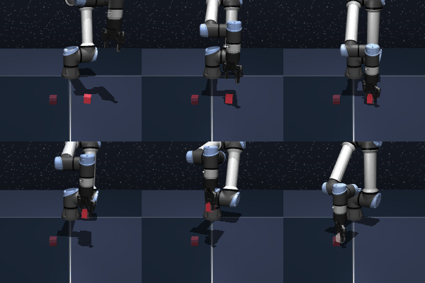
The tasks are from OGBench: cube-single-play (pick up a cube and place it at a goal) and antsoccer-arena-navigate (a quadruped dribbles a ball to a goal, more long-horizon). Both are single-task with 1M gradient steps.
Results
| cube-single | antsoccer-navigate | |
|---|---|---|
| SAC+BC | 1.00 (\(\alpha = 300\)) | 0.32 (\(\alpha = 3\)) |
| IQL | 0.92 (\(\alpha = 30\)) | 0.20 (\(\alpha = 10\)) |
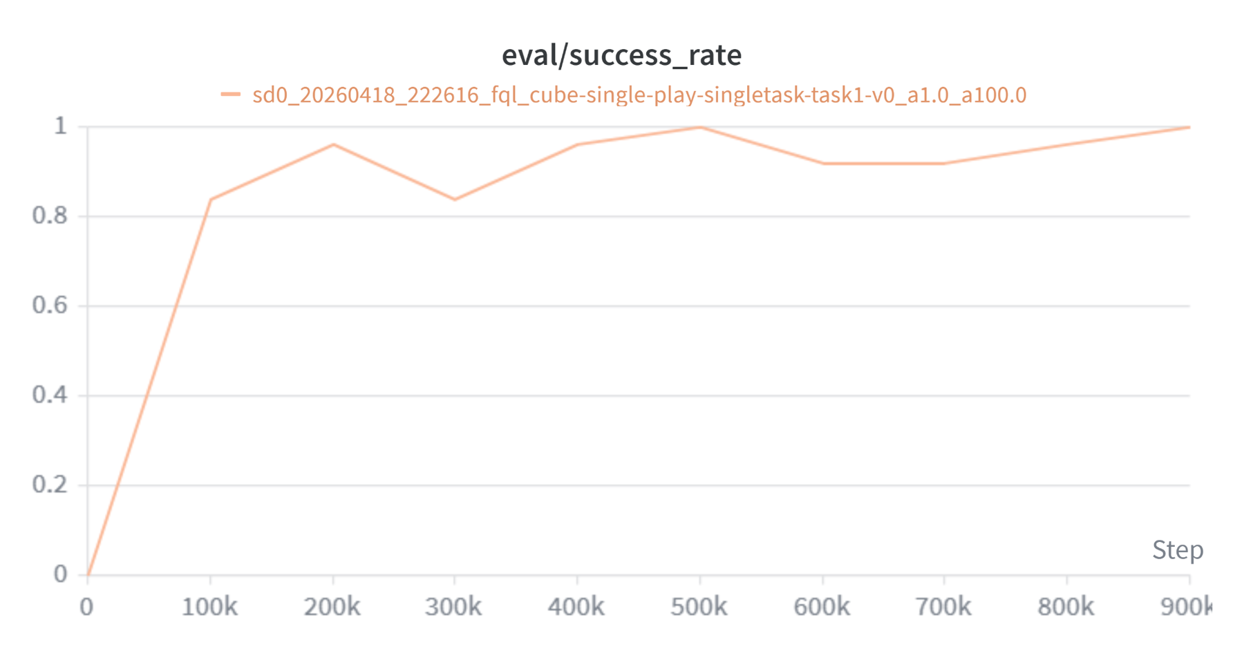
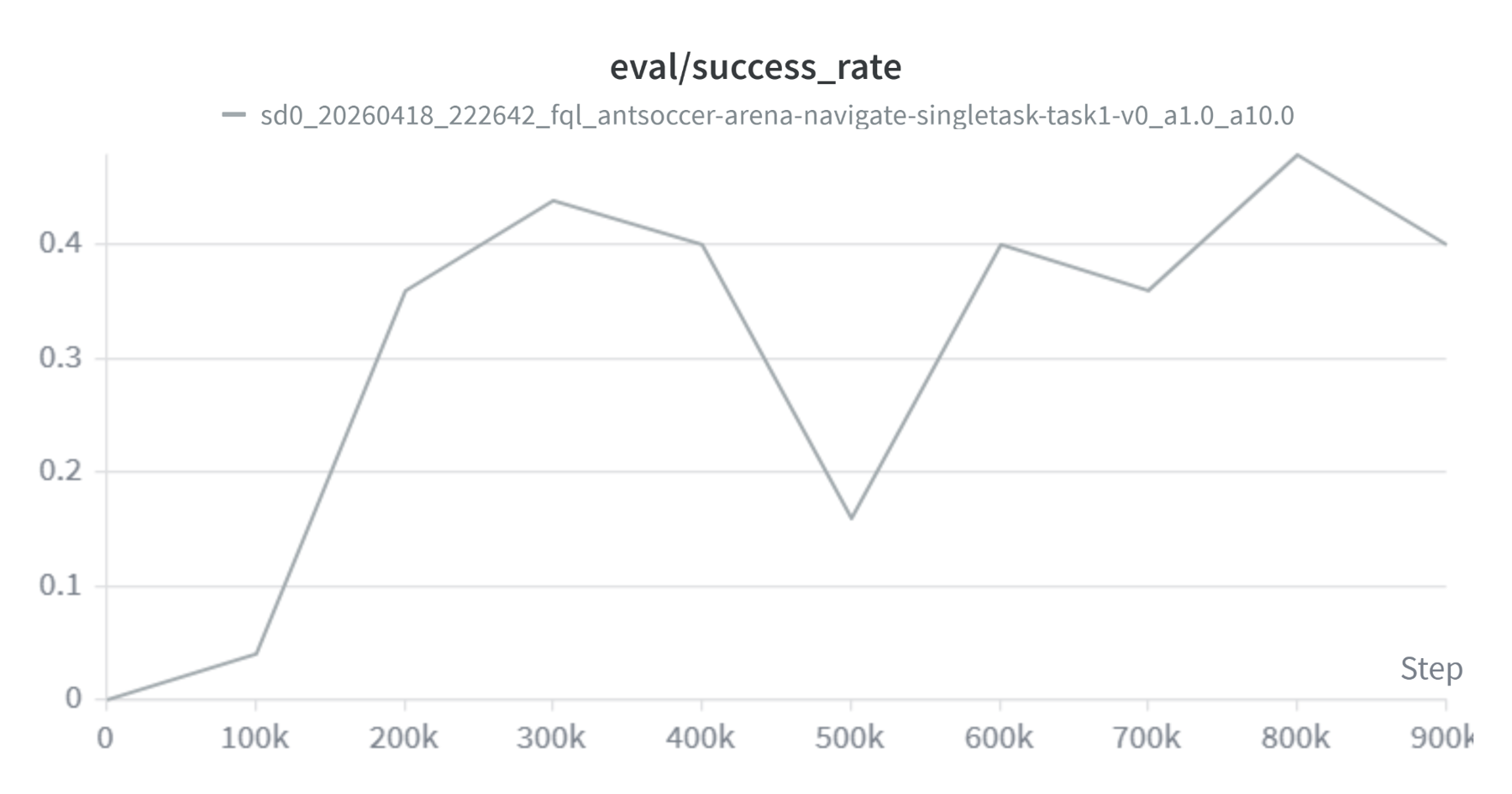
| FQL | 1.00 (\(\alpha = 100\)) | 0.48 (\(\alpha = 10\)) |
All 3 methods nearly solve cube. On antsoccer FQL does best, at about 0.48.
Hyperparameter sensitivity
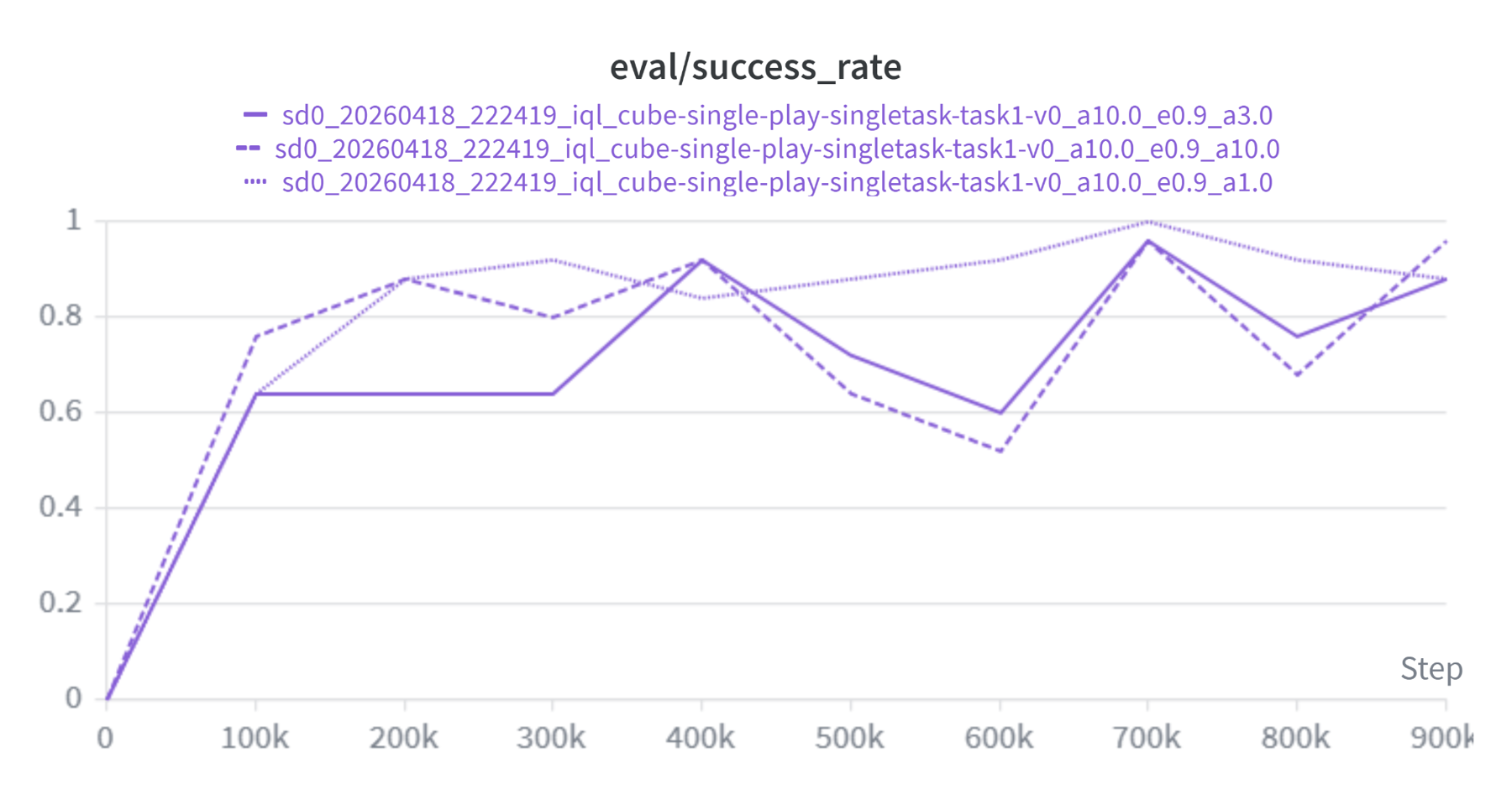
I swept each method’s main hyperparameter on cube-single.
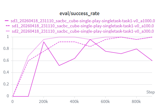
SAC+BC is sensitive to \(\alpha\). \(\alpha = 100\) and 300 both reach about 1.0, but \(\alpha = 1000\) peaks at 0.92 and then drops to 0.6. With too much BC weight the actor imitates the play data, which wasn’t collected for this task. With too little it exploits the critic’s errors. The best value also differed by 100× between tasks (300 on cube, 3 on antsoccer).
IQL is much less sensitive. Across a 10× range of \(\alpha\) the 3 curves stay in the same 0.6–1.0 band and cross each other repeatedly. IQL only evaluates Q at dataset actions, so \(\alpha\) only changes how strongly it weights the better dataset actions, and the policy can’t move outside the data. This also limits IQL to reweighting the data, and it had the lowest score on antsoccer.
The 3 SAC+BC runs used different seeds, so the \(\alpha = 1000\) drop could partly be a seed effect. I’d need several seeds per setting to say more.
Flow Q-learning
FQL addresses a problem from Push-T: the best BC policies are expressive generative models such as flow and diffusion heads, and these are hard to train with RL. Their likelihood is intractable, so AWR doesn’t apply, and maximizing Q directly requires backpropagating through the ODE solve, which is slow and unstable.
FQLPark, Li & Levine, Flow Q-Learning, ICML 2025. avoids both problems:
- Train a flow-matching BC policy \(\mu_\beta(s, z)\) on the dataset. It can represent multiple modes and is never trained on Q.
- Train a separate one-step policy \(\mu_\omega(s, z)\), mapping noise directly to an action, with \(\mathcal{L}(\omega) = -Q\big(s, \mu_\omega(s, z)\big) + \alpha\,\big\lVert \mu_\omega(s, z) - \mu_\beta(s, z)\big\rVert^2 .\)
The distillation term keeps the one-step policy close to the BC policy for the same noise \(z\). Different noise still maps to different modes, and Q moves each sample toward better actions within its mode. No gradient goes through the ODE, so the RL update costs about the same as SAC+BC.