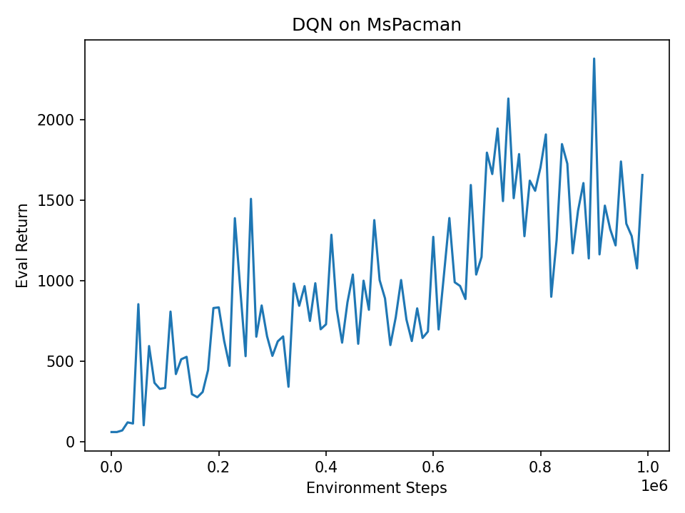
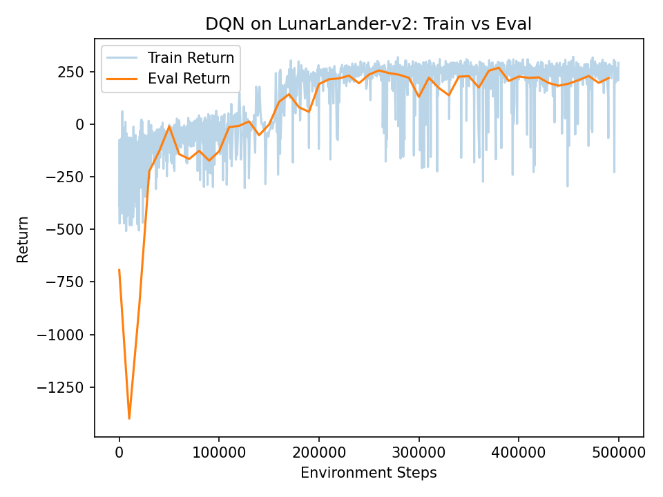
Policy gradients use each sample for one update and then discard it. Value-based methods keep a replay buffer and regress a Q-function onto bootstrapped targets, which is much more sample efficient, but the network is trained on its own predictions. This post covers the problems that causes and the fixes DQN and SAC use.
DQN
The Q-learning target is \(y = r + \gamma \max_{a'} Q_{\bar\phi}(s', a')\), where \(\bar\phi\) is a slowly updated target network. On CartPole, plain DQN learns quickly but doesn’t stay stable:
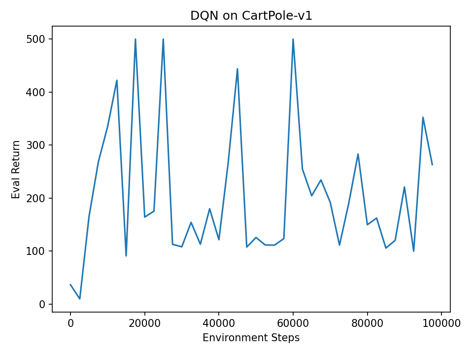
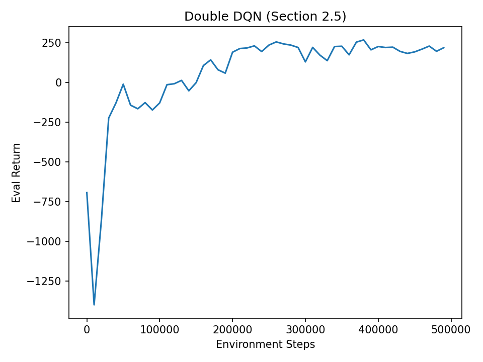
The CartPole instability is an example of the deadly triadSutton & Barto, Reinforcement Learning: An Introduction, §11.3.: function approximation, bootstrapping, and off-policy data. Every Q update moves the targets of every other state. The \(\max\) makes this worse because it selects the action whose estimate is most overestimated, and bootstrapping compounds that bias. Double DQN decouples choosing the action from evaluating it, using \(y = r + \gamma\, Q_{\bar\phi}(s', \arg\max_{a'} Q_\phi(s', a'))\). The online network picks the action and the target network scores it, so the 2 have to be wrong in the same direction for the error to propagate.
max estimator: pick and score with the same estimatedouble estimator: pick with A, score with B
SAC
For continuous actions you can’t take a \(\max\) over \(a'\), so you learn a policy that does the maximizing. Soft actor-critic adds an entropy bonus to the objective, so the critic learns soft Q-values:
\[y = r + \gamma\Big(\min_{j=1,2} Q_{\bar\phi_j}(s', a') - \alpha \log \pi(a' \mid s')\Big), \quad a' \sim \pi(\cdot \mid s'),\]and the actor minimizes \(\mathbb{E}\big[\alpha \log\pi(a \mid s) - Q(s, a)\big]\) with reparameterized samples \(a = \tanh(\mu_\theta(s) + \sigma_\theta(s)\,\epsilon)\).
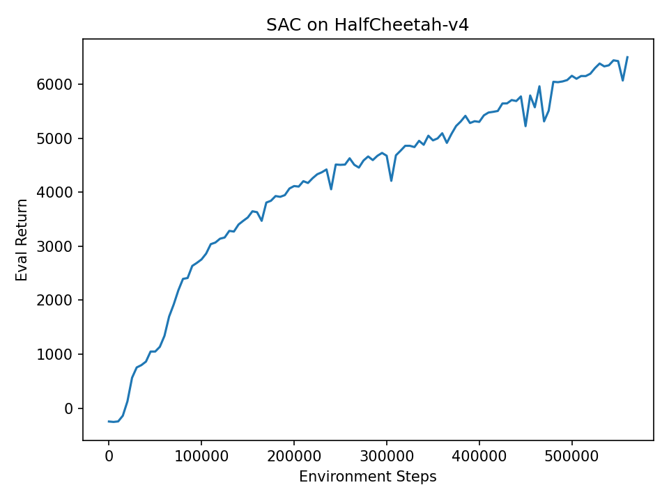
Clipped double-Q
The \(\min\) over 2 critics in the target is SAC’s version of the double DQN fix. Removing it on Hopper had the largest effect of any change in this homework:
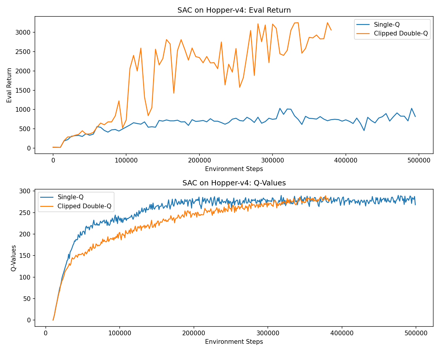
With a single critic, Hopper plateaus around 750. With clipped double-Q it reaches 2500–3200. In the bottom plot, the single critic reports higher Q-values than the clipped one for the first 300k steps, even though its policy is much worse, so those values are overestimates. The actor moves toward actions whose values are inflated, which reinforces the error. Taking the minimum of 2 independently initialized critics is a simple form of pessimism that counters this.
Auto-tuned temperature
Instead of fixing \(\alpha\), SAC can treat it as a Lagrange multiplier on an entropy constraint \(\mathbb{E}[-\log\pi] \ge \bar{\mathcal{H}}\) (the target is usually \(-\lvert\mathcal{A}\rvert\)) and learn it by gradient descent on \(\alpha\,(-\log\pi - \bar{\mathcal{H}})\).
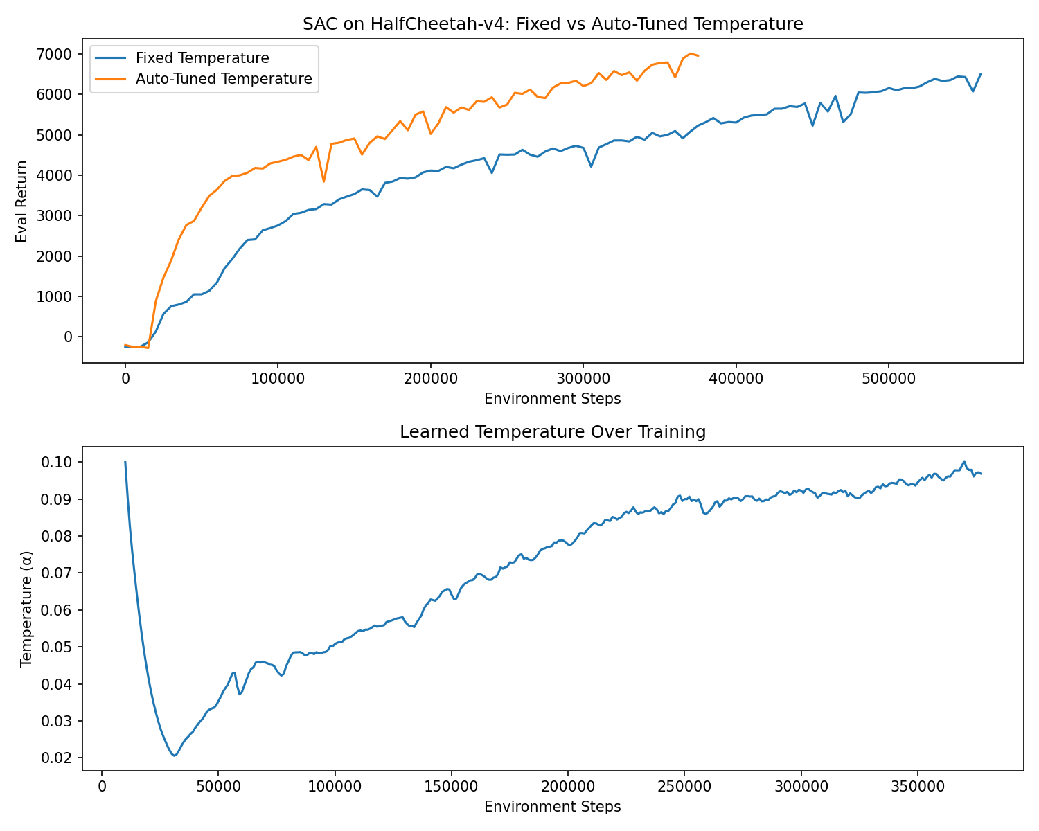
The entropy constraint:
- Early: the policy is close to its initialization, so its entropy is well above the target. The constraint is slack, so gradient descent lowers \(\alpha\) quickly over the first 30k steps.
- Later: as the critic learns, Q-values grow (this is a dense reward task with returns in the thousands), and the gradient of \(-Q\) increasingly dominates the actor loss. The policy sharpens, its entropy drops below the target, and \(\alpha\) rises to push it back up.
The rising \(\alpha\) compensates for the growing reward scale, which would otherwise make the policy’s entropy collapse. With a fixed \(\alpha\), the entropy term becomes relatively weaker as Q-values grow, which is probably why the fixed run learns more slowly.