Policy gradients, one variance reduction at a time

The policy gradient is

\[\nabla_\theta J(\theta) = \mathbb{E}_{\tau \sim \pi_\theta}\Big[\sum_{t} \nabla_\theta \log \pi_\theta(a_t \mid s_t)\; \hat A_t\Big].\]

Much of on-policy RL comes down to the choice of \(\hat A_t\), which trades off bias and variance. The vanilla estimator is unbiased but has high variance. Each technique below reduces variance, and the later ones introduce some bias to do so.

Reward-to-go

Vanilla REINFORCE weights every \(\log\pi(a_t \mid s_t)\) by the return of the whole trajectory, \(\sum_{t'} r_{t'}\). But rewards before time \(t\) can’t depend on \(a_t\), so in expectation they contribute zero gradient and only add noise. Dropping them gives reward-to-go, \(\hat Q_t = \sum_{t' \ge t} \gamma^{t'-t} r_{t'}\). It is still unbiased, and each term is now a sum over fewer random rewards.

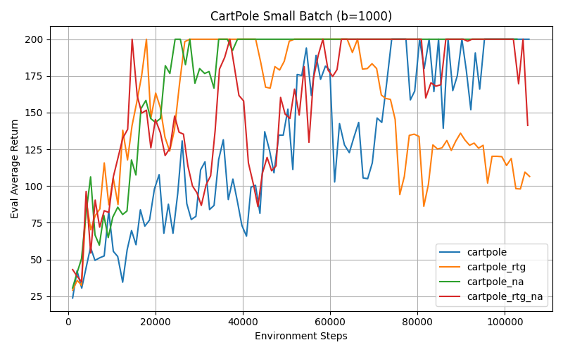
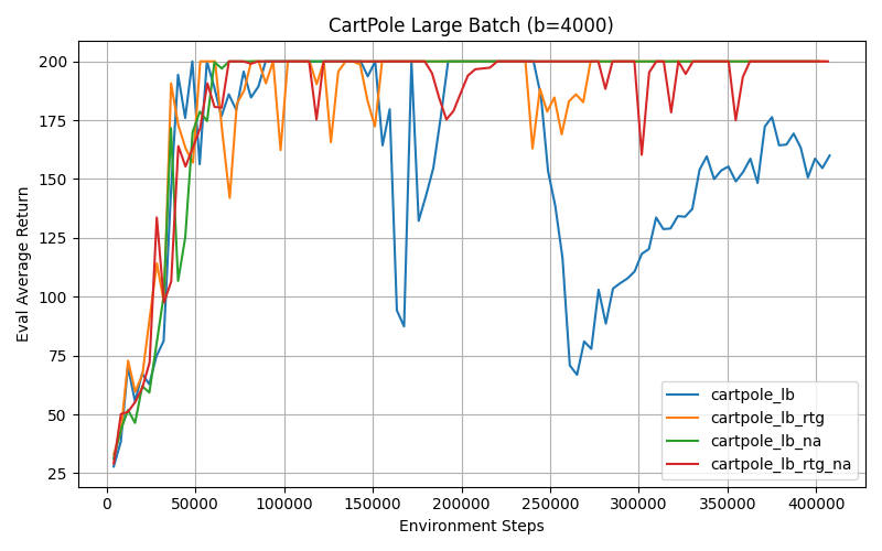
CartPole learning curves with batch size 4000 for the same 4 variants. — CartPole with batch size 1000 (left) and 4000 (right).

On CartPole, reward-to-go beat the trajectory-centric estimator. Normalizing advantages (subtracting the batch mean and dividing by the std) helped both: it acts like a per-batch learning-rate adjustment and keeps the gradient scale consistent. A bigger batch smoothed everything out. With 4000 steps per update, everything except vanilla REINFORCE sits at 200 almost the whole time. Vanilla REINFORCE with the large batch still collapses twice, at about 170k and 265k steps, and doesn’t fully recover from the second. A larger batch reduces variance but doesn’t fix the estimator.

A learned baseline

Subtracting any function of the state leaves the gradient unbiased, since \(\mathbb{E}_{a}[\nabla \log \pi(a \mid s)\, b(s)] = 0\).Because \(\mathbb{E}_{a \sim \pi}[\nabla_\theta \log \pi_\theta(a \mid s)] = \nabla_\theta \sum_a \pi_\theta(a \mid s) = \nabla_\theta 1 = 0\), and \(b(s)\) factors out of the expectation over \(a\). A common choice is \(b(s) \approx V^\pi(s)\), which turns \(\hat Q_t\) into an advantage. I fit \(V_\phi\) by regression on the reward-to-go and compared the default baseline (lr 0.01, 5 gradient steps per iteration) to a weaker one (lr 0.001, 1 step).

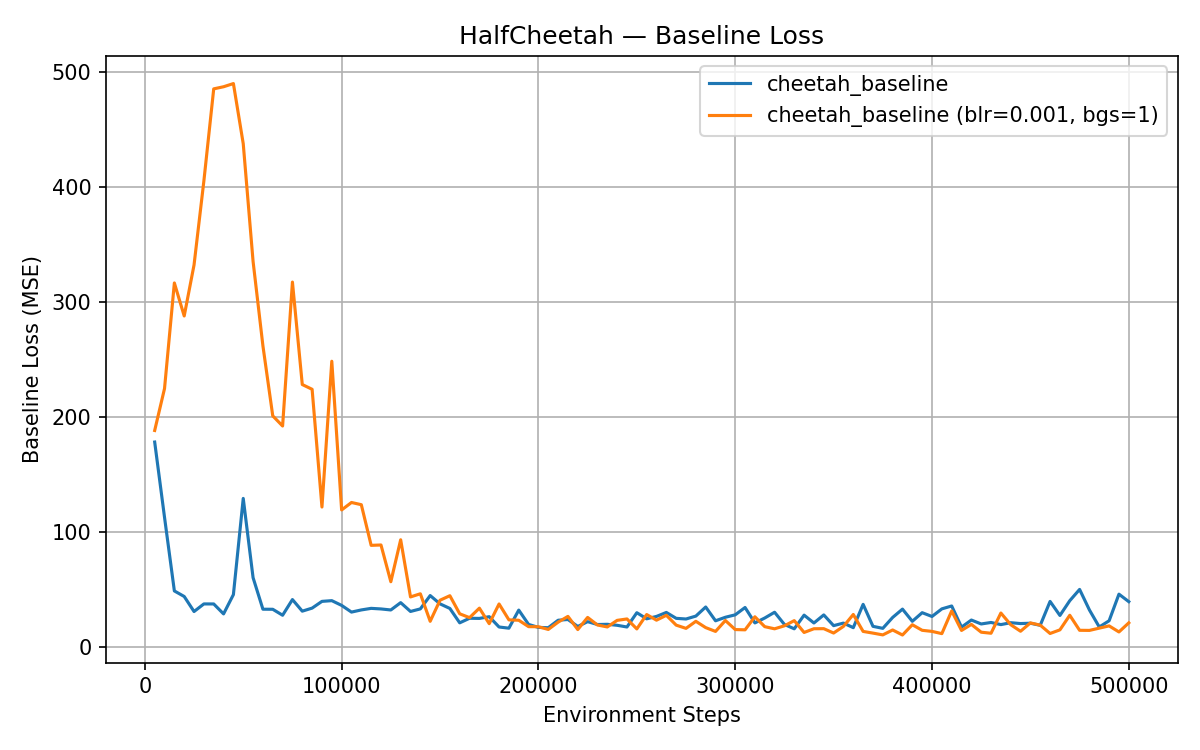
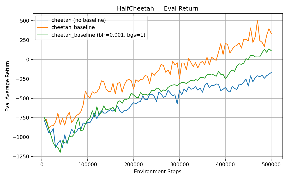
Value function MSE over training for default and weak baselines; the weak baseline has a large early spike. — HalfCheetah. Left: the weak baseline's value loss spikes to almost 500 early and takes about 150k steps to catch up. Right: no baseline < weak baseline < default baseline, in that order, for essentially the whole run.

HalfCheetah eval return: default baseline highest, weak baseline in between, no baseline lowest. — HalfCheetah. Left: the weak baseline's value loss spikes to almost 500 early and takes about 150k steps to catch up. Right: no baseline < weak baseline < default baseline, in that order, for essentially the whole run.

A value function that tracks \(V^\pi\) poorly subtracts the wrong amount, so the advantage estimates have more variance and the policy learns more slowly. Even the weak baseline is much better than none.

GAE: interpolating between Monte Carlo and TD

Once you have \(V_\phi\) you can also bootstrap with it. Generalized advantage estimation takes an exponentially weighted average of \(n\)-step advantages:

\[\hat A_t^{\text{GAE}(\lambda)} = \sum_{l \ge 0} (\gamma\lambda)^l\, \delta_{t+l}, \qquad \delta_t = r_t + \gamma V_\phi(s_{t+1}) - V_\phi(s_t).\]

At \(\lambda = 0\) this is the one-step TD advantage \(\delta_t\). At \(\lambda = 1\) you get reward-to-go minus the baseline.

How much GAE(λ) trusts each future TD error

GAE(λ) weightsλ = 1 (Monte Carlo)

γ λ

LunarLander eval return for lambda in 0, 0.95, 0.98, 0.985, 0.99, 1. — LunarLander-v2 for six values of \(\lambda\).

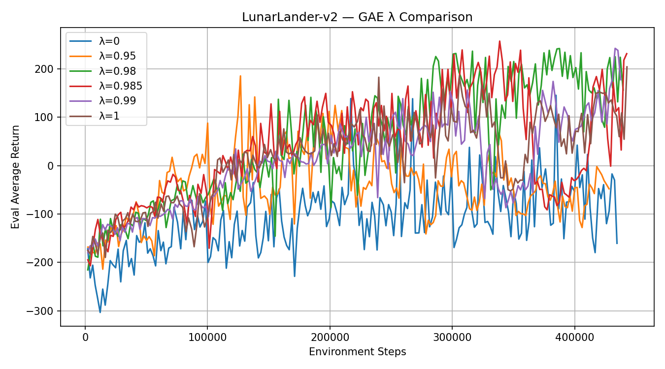
\(\lambda = 0\) (blue) is the worst performing. It hovers around −100 to 0 for the whole run, because \(V_\phi\) is inaccurate early in training and \(\lambda = 0\) relies on it entirely. The intermediate values, 0.95 to 0.99, are the ones that reach +200, with \(\lambda = 0.98\) the most stable. \(\lambda = 1\) gets there too but is noisier. The best values are close to 1, which fits LunarLander’s long episodes.

InvertedPendulum

The last task was to get InvertedPendulum to its maximum return of 1000 within 100k environment steps.

uv run src/scripts/run.py --env_name InvertedPendulum-v4 -n 100 \
    -b 1000 -eb 1000 -rtg -na -lr 0.02

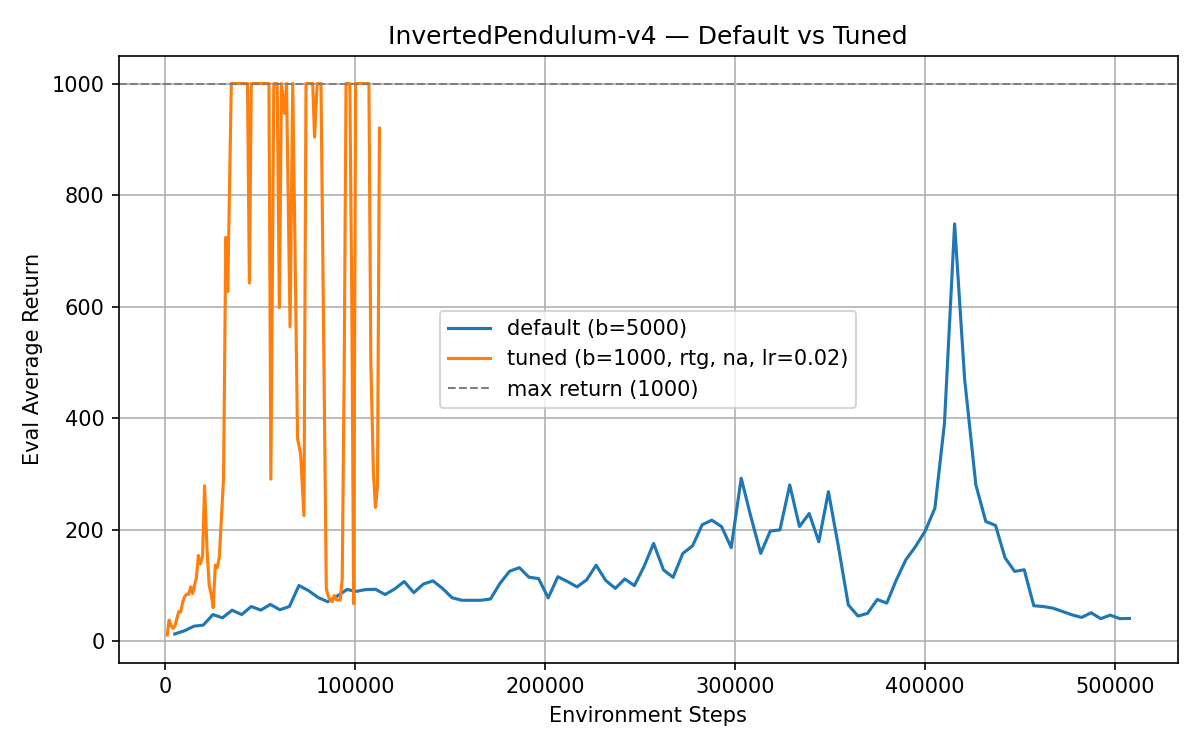
InvertedPendulum: default config stays under 300 for most of 500k steps; tuned config hits 1000 by around 40k steps but oscillates. — Default (blue) vs. tuned (orange). The tuned run first hits 1000 at about 35k steps.

The batch size mattered most. With the default 5000 steps per iteration, a 100k-step budget is 20 gradient updates. With 1000 it is 100 updates. Reward-to-go and advantage normalization made the noisier updates usable, and raising the learning rate from 0.005 to 0.02 made each update larger.

The policy isn’t stable, though. The tuned run keeps dropping below 1000 and recovering, since a large step size with a high-variance gradient occasionally produces a bad update.