Push-T is a standard benchmark for visuomotor imitation learning. A circular agent pushes a T-shaped block into a target pose, and the policy is trained on a set of expert demonstrations. The task is simple, but it requires a policy that can represent an action distribution with more than one mode.
I trained 2 policies on the same demos with the same budget. One regresses action chunks with MSE. The other samples action chunks with flow matching. The flow policy reached a mean reward of 0.82, and the MSE policy plateaued around 0.67. This post aims to explain the gap.
Setup
- State: \(s \in \mathbb{R}^5\) (agent position plus block pose).
- Action: a chunk of 8 future 2D agent targets, \(a \in \mathbb{R}^{8 \times 2}\).Action chunking was popularized by ACT (Zhao et al., 2023) for bimanual manipulation. Predicting chunks instead of single actions gives temporally consistent motion and fewer chances to switch between strategies at every step.
- Training: 400 epochs (75,600 gradient steps) for both policies, with evaluation every 10k steps.
The MSE policy
A 3-layer MLP (256 hidden units, ReLU) maps the state to a flattened \(8 \times 2\) chunk, trained with MSE using Adam at 3e-4 and batch size 128.
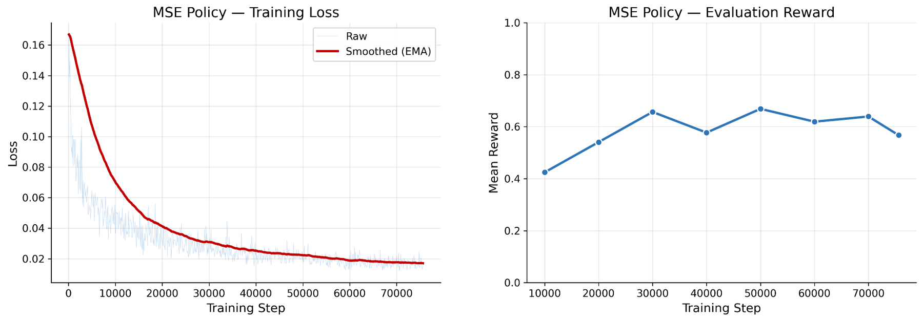
The training loss keeps decreasing, but MSE doesn’t measure what we want. The minimizer of the squared error is the conditional mean:
\[\pi_{\text{MSE}}^*(s) = \arg\min_{\hat a}\; \mathbb{E}_{a \sim \pi_E(\cdot \mid s)} \lVert a - \hat a \rVert^2 = \mathbb{E}[a \mid s].\]In Push-T the expert’s action distribution is often bimodal. From the same state, the demonstrator can go around the left side of the T or the right side to get behind it. Both work, but their average sends the agent into the middle of the block or leaves it between the 2 plans. The rollouts show this: hesitant pushes and contact that slides off.
The demo below shows this in a toy 2D action space. The gray points are expert actions for a single state, split between 2 modes. On the left is where an MSE regressor ends up. On the right, noise is transported to actions by the flow-matching velocity field for this distribution.
expert actionsMSE predictionflow samples
The flow matching policy
Flow matching learns a velocity field \(v_\theta(a_t, t \mid s)\) that transports Gaussian noise into the action distribution. To train it, take an expert chunk \(a_1\) and noise \(\varepsilon\), set \(a_t = (1-t)\,\varepsilon + t\,a_1\) (noise at \(t = 0\), data at \(t = 1\)), and regress
\[\mathcal{L}(\theta) = \mathbb{E}_{t,\,a_1,\,\varepsilon}\,\big\lVert v_\theta(a_t, t \mid s) - (a_1 - \varepsilon)\big\rVert^2 .\]This is still an MSE loss, so it still learns a conditional mean. The difference is what it conditions on. The flow model regresses the mean velocity given a partially denoised \(a_t\). Near \(t = 0\) that mean averages over both modes, but as \(a_t\) drifts toward one of them the conditional collapses onto that mode. The averaging happens in velocity space at each point along the path, not in action space at the end. At test time I integrate the ODE forward from \(t = 0\) to 1 starting from fresh noise, so different noise draws commit to different modes.
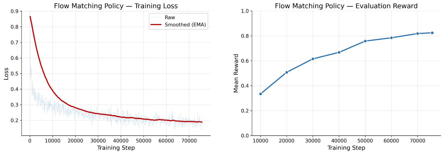
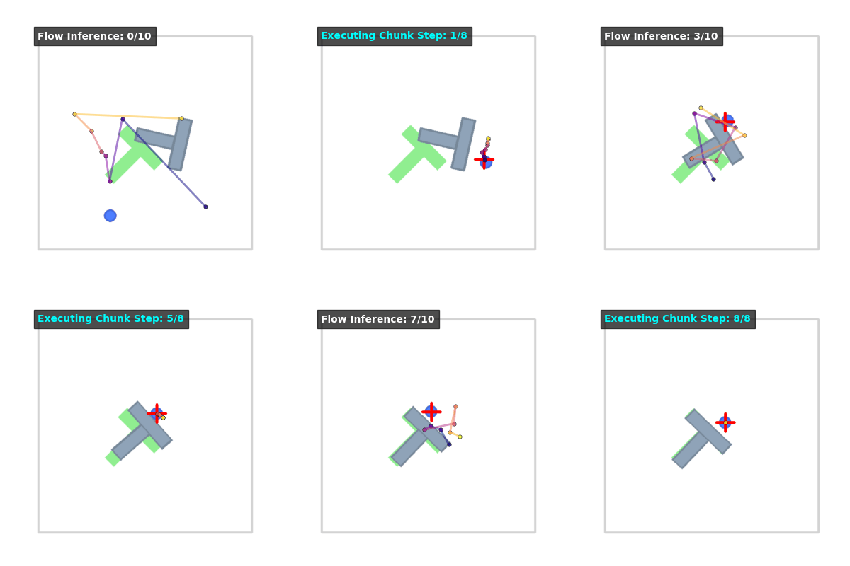
The rollouts match the numbers: the flow policy commits to one strategy and its pushes make clean contact. The MSE policy’s pushes look tentative, consistent with averaging between strategies.
Summary
- Multimodal action distributions are common in manipulation (grasping from either side, going around either way, using either hand), which is a large part of why Diffusion Policy and flow-matching action heads like \(\pi_0\)’s are widely used.
- The flow head has a downside. Its likelihood is intractable, and maximizing a Q-function through it means backpropagating through an ODE solve. That is the main obstacle to doing RL on top of these policies. So VLA RL requires some modifications.