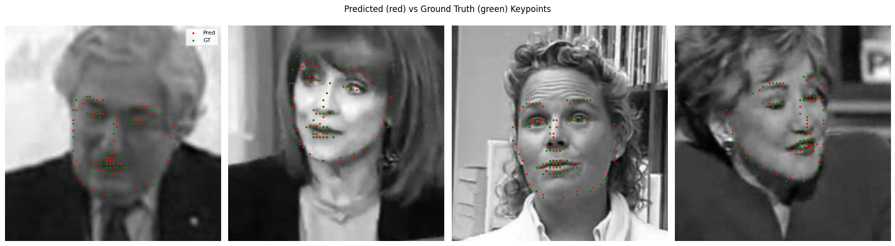
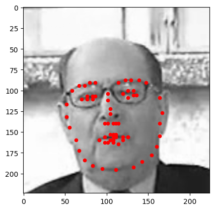
The task is to predict 68 landmarks (jaw, brows, eyes, nose, mouth) as \((x, y)\) pairs from a 224×224 grayscale face. I tried 3 approaches: regressing coordinates directly, fine-tuning pretrained backbones, and predicting heatmaps.
| Approach | Test MSE ↓ |
|---|---|
| CNN, direct coordinate regression | 0.0459 |
| ResNet-18 (ImageNet), frozen then fine-tuned | 0.0076 |
| DINOv2 ViT-S/14, frozen then fine-tuned | 0.0099 |
| U-Net heatmaps + argmax | 0.0147 (val 0.0007) |
1. Regressing coordinates directly
A 4-block CNN (32 to 256 channels, BatchNorm, max pool, increasing dropout) followed by an MLP head that outputs 136 numbers, trained with SmoothL1. A small sweep over learning rate, loss, and activation favored lr 1e-3, SmoothL1 over MSE (less sensitive to wrong labels), and ELU over ReLU.
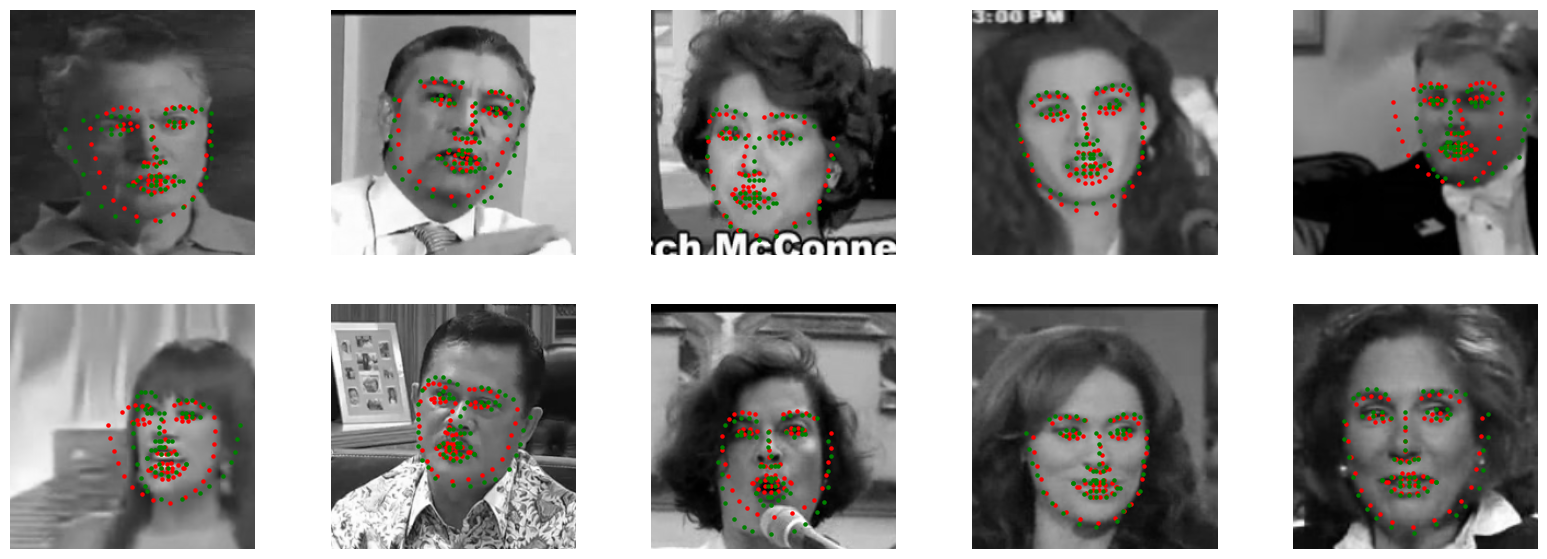
This has the same problem as MSE action regression: when the regressor is unsure about the pose, it predicts something close to the mean face, placed roughly in the right location. Also, 51M of the network’s parameters are in the first fully connected layer, which has to learn spatial reasoning from a flattened feature map.
2. Transfer learning
ResNet-18. I replaced the first conv with a 1-channel version, initialized by averaging the pretrained RGB filters so the pretrained edge filters are kept. I put a small MLP head on top and trained in 2 phases: 15 epochs freezing everything except the input conv and head, then 20 epochs end to end with a 4× smaller learning rate on the backbone.
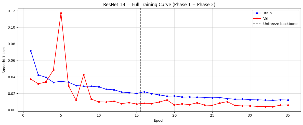
This reduced test MSE from 0.046 to 0.0076, a 6× improvement, and removed most of the large failures. ImageNet features already encode edges and object parts, so the head only has to map them to coordinates.
DINOv2 (ViT-S/14, CLS token to linear head) reached 0.0099 and was the hardest to train. Phase 1 (frozen backbone) barely improved, and phase 2 needed a backbone learning rate of 2e-6 to avoid degrading the features. I think regressing from the CLS token was the main problem. B/c it’s a global summary trained to be invariant to the kind of spatial detail this task needs, and the patch tokens carry more localization information.
3. Heatmaps
Instead of 136 numbers, predict 68 images: a U-Net outputs a 64×64 heatmap per keypoint, trained with MSE against a Gaussian (σ = 2) placed at the true location. Coordinates come from the argmax.
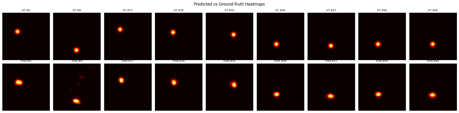
This parameterization suits a conv net. The output is in the same spatial frame as the input, so translation equivariance handles what the regression MLP had to learn. A heatmap can also be bimodal when the model is unsure, and the argmax picks one mode instead of averaging them, similar to flow vs. MSE policies. Training was the most stable of the 4.