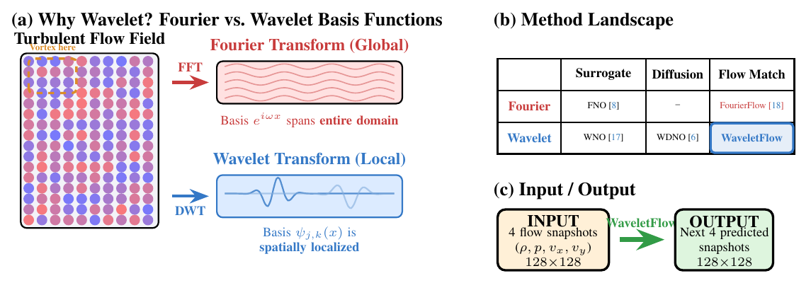
The problem of spectral bias
Diffusion and flow models recover coarse, low frequency structure first and fine, high frequency structure last. High frequencies therefore drop below the noise floor earliest in the forward process, and the reverse process has the least signal to recover them from. For turbulence that is bad news, because the vortices and shear layers carrying the interesting physics live at high wavenumbers.
FourierFlow (Wang et al.) addressed this with a learnable spectral filter weighted by \(\lVert\xi\rVert^\eta\), which pushes the model toward high frequencies. However this filter is global. Turbulent fields are mostly smooth with a few localized vortex cores, so amplifying a certain frequency band amplifies the quiet regions too.
WaveletFlow Architecture
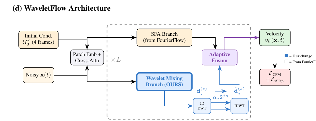
We swapped FourierFlow’s Fourier Mixing branch for a Wavelet Mixing branch and also modified the salient-flow attention branch, the conditioning, the gated fusion, and the MAE alignment loss.
- Take a 2-level 2D DWT of the feature map.
- At each level, run the 3 detail subbands (LH, HL, HH) through a per-level MLP.
- Rescale each level by \(\beta_j + \alpha_j 2^{j\eta_j}\). This plays the role of \(\lVert\xi\rVert^\eta\), but acts on spatially indexed coefficients.
- Run the inverse DWT with the approximation coefficients untouched, and add residual.
Results
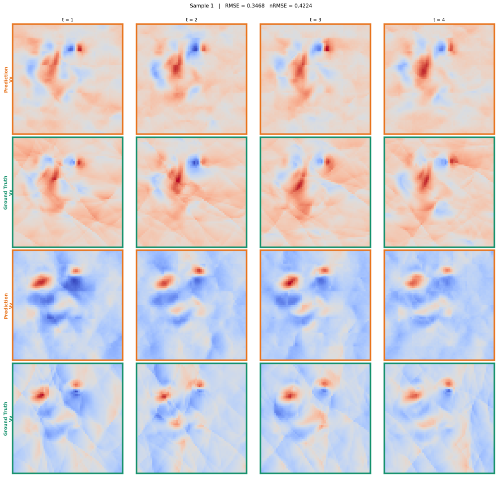
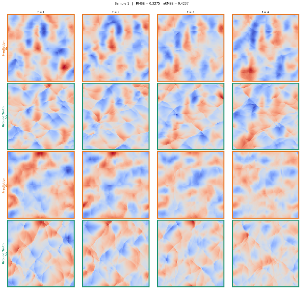
On PDEBench compressible Navier–Stokes, we tested both models trained under the same reduced budget:
| Method | RMSE ↓ | nRMSE ↓ | vs. FourierFlow |
|---|---|---|---|
| FourierFlow | 0.3225 | 0.4201 | |
| WaveletFlow (db4) | 0.2955 | 0.3924 | −8.4% RMSE |
| WaveletFlow (Haar) | 0.2974 | 0.3865 | −7.8% RMSE |
db4 has smoother, longer filters and better frequency selectivity, which suits absolute error. Haar has the most compact support, and gets the best normalized error, which fits a field whose hard parts are sharp and spatially concentrated.
Caveats
The original FourierFlow was trained on 8×H800s for a long time. We trained both models with fewer epochs and smaller batches on 3×RTX 6000 Ada. The comparison is fair under that budget, but it isn’t a reproduction of the published numbers.