A diffusion or flow model trained perfectly on a finite dataset can only reproduce the training set: the optimal velocity field for an empirical distribution transports every noise sample onto one of the training points. Trained models do generate new samples, so their ability to generalize has to come from the ways they differ from the optimal field.
Kamb & Ganguli (2024) provide a clean proof of this phenomenon for UNet denoisers. They build analytic, training-free “score machines” with the inductive biases of a CNN (locality and translation equivariance) and show that they predict what a trained convolutional diffusion model generates from a given noise sample. In CS 280 we reimplemented these machines for flow matching and compared them against a UNet we trained ourselves, from identical noise.
Part 1: one-step denoising
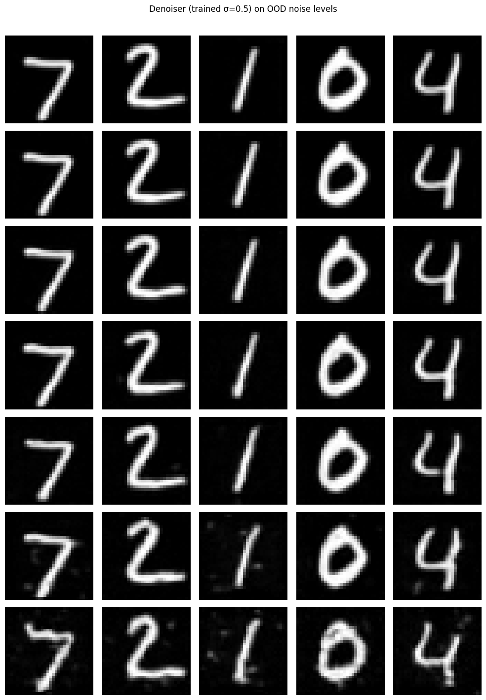
Before the flow model I trained a plain denoiser \(D(z) \approx x\) on MNIST digits with noise \(\sigma = 0.5\) added. It’s just a small UNet trained with an L2 loss.
To make it generative in one step, I trained the same network to map pure noise \(\varepsilon \sim \mathcal{N}(0, I)\) directly to a digit.

The L2-optimal predictor is \(\mathbb{E}[x \mid z]\). When \(z\) is pure noise it carries no information about \(x\), so \(\mathbb{E}[x \mid z] = \mathbb{E}[x]\) and the network outputs the dataset mean, which looks like every digit superimposed. Indeed, MSE tends to be mean seeking. Iterative denoising avoids it by conditioning on a partially denoised \(x_t\) and taking small steps, so each step predicts the mean of a narrower distribution.
Part 2: flow matching
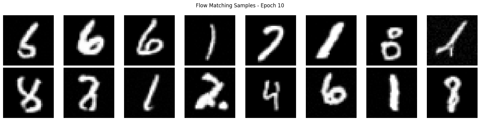
With \(x_t = (1-t)\,\varepsilon + t\,x_1\) (noise at \(t=0\), data at \(t=1\)), the UNet takes the time as a sinusoidal embedding and regresses the velocity \(x_1 - \varepsilon\). Sampling is just Euler integration from \(t=0\) to 1.I use the Lipman et al. convention throughout this post. Kanazawa used the reverse, with data at \(t = 0\), which is why the noise image is labeled \(x_1\).
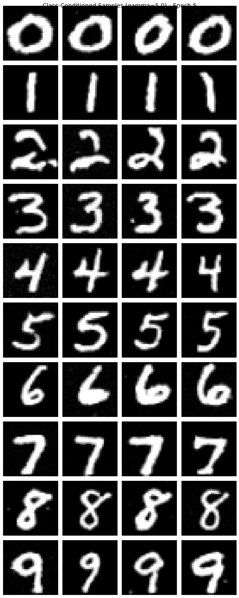
Adding a class embedding with 10% label dropout gives classifier-free guidance, \(v = v_\varnothing + \gamma\,(v_c - v_\varnothing)\):
Part 3: the ideal flow
For a finite training set \(\{p^{(i)}\}\), the optimal velocity has a closed form. Given \(x_t = a_t x_1 + b_t \varepsilon\) with \(a_t = t\) and \(b_t = 1 - t\), the posterior over which training point we came from is a softmax over distances:
\[w_i(x, t) \propto \exp\!\left(-\frac{\lVert x - a_t\, p^{(i)}\rVert^2}{2 b_t^2}\right), \qquad \hat x_1 = \sum_i w_i\, p^{(i)},\]and the velocity is \(v = \mathbb{E}[x_1 - \varepsilon \mid x_t] = \frac{\hat x_1 - x}{1 - t}\), which points toward the posterior mean with speed increasing as \(t \to 1\). As \(t \to 1\) the softmax also sharpens onto a single \(p^{(i)}\), and the sample lands exactly on it. In the demo below you can click to add training points.
training pointssamples
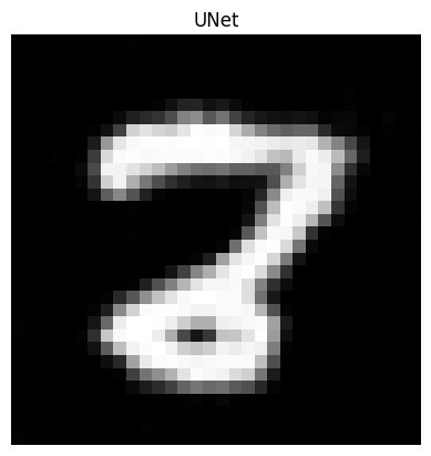
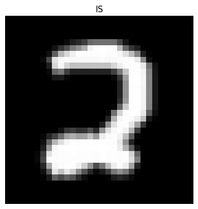
This is the IS (ideal score) machine. On MNIST, from our noise sample, it produces a 2 that is an exact copy of a training image. The UNet produces a different image from the same noise.
Part 4: IS, LS, ELS, bbELS
Kamb & Ganguli make the posterior local. Each pixel only gets to look at a \(k \times k\) patch around itself, and the softmax runs over training patches instead of whole images. For pixel \(u\), with \(x_{\Omega_u}\) the patch around it:
\[\ell(p) = -\frac{\lVert x_{\Omega_u} - a_t\, p \rVert^2}{2 b_t^2}, \qquad \hat x_1(u) = \frac{\sum_p e^{\ell(p)}\, p_{\text{center}}}{\sum_p e^{\ell(p)}}.\]Every pixel independently picks the training patches that best explain its neighborhood and copies their center pixel. Different pixels can copy from different images. This allows new combinations that are locally consistent with the training data but aren’t copies of any one image. The 4 machines differ only in which patches each pixel is allowed to compare against.
| Machine | Patches | Compared against | Inductive bias |
|---|---|---|---|
| IS | the whole image | whole training images | none (memorizes) |
| LS | \(k \times k\) | training patches at the same location | locality |
| ELS | \(k \times k\) | training patches at any location | locality + translation equivariance |
| bbELS | \(k \times k\) | any location, but border patches only match border patches with the same overlap | + the boundary breaks equivariance |
The patch size \(k\) follows a schedule over time: small at low noise and large at high noise, ranging from 3 to 27 here. The reason is that a UNet’s effective receptive field grows with the noise level. In the implementation, everything is a softmax-weighted average over millions of patches (10k images × 1024 positions).For ELS, every pixel compares against all ~10M training patches at every one of the 20 steps.
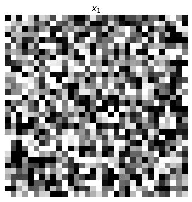 noise \(\varepsilon\)
 UNet
 IS
 LS
 ELS
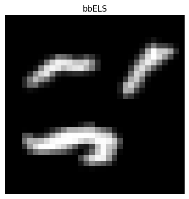 bbELS
Results
The results only partly matched the paper.
- IS copied a training image, as expected.
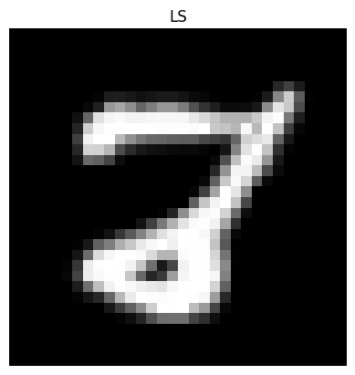
- LS gave the closest match to the UNet: a single connected stroke in roughly the right place, with the same loop at the bottom. MNIST digits are centered, so comparing only against patches at the same location is a good prior for this dataset.
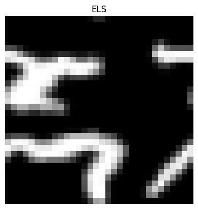
- ELS and bbELS produced collages of plausible stroke fragments that don’t form a digit. Each patch is locally reasonable, but nothing coordinates them globally. The boundary-broken version clears up the borders as intended, but the interior stays fragmented.